Convolution Vs Correlation

Concept of Linear Convolution

The concept of convolution is central to Fourier theory and the analysis of Linear Systems. In fact the convolution property is what really makes Fourier methods useful. In one dimension the convolution between two functions, f (x) and h(x) is defined as:

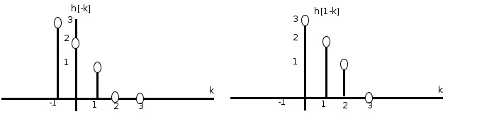
Where ‘s’ is a dummy variable of integration. This operation may be considered the area of overlap between the function f(x) and the spatial (or time) reversed version of the function h(x). For discrete signals the integration in above equation is replaced by summation. The result of the convolution of two simple one dimensional functions is shown in figure 1.

 

The Convolution theorem relates the convolution between the two real space (or time) domain signals to a multiplication in the Fourier domain, and can be written as;

                                                          
                                                           
Convolution Properties

The convolution is a linear operation which is distributive, so that for three functions f (x), g(x) and h(x) we have that

                                        

and commutative, so that

If the two functions f (x) and h(x) are of finite extent, (are zero outside a finite range of x), then the extent (or width) of the convolution g(x) is given by the sum of the widths the two functions. For example if figure 1 both f (x) and h(x) non-zero over the finite range x = ±1. Thus the convolution g(x) is non-zero over the range x = ±2. If f[n] and h[n] are two finite length sequences of lengths L₁ and L₂ then g[n] will be of length L₁+L₂-1.

Correlation of two Signals

A closely related operation to Convolution is the operation of Correlation of two functions. In Correlation two functions are shifted and the area of overlap formed by integration, but this time without the spatial (or time) reversal involved in convolution. The Correlation between two function f (x) and h(x) is given by

                                   

This is for real signals, for complex signals h^*(s-x) is used, where h^*(x) is the complex conjugate of h(x). This operation is shown for two simple functions in figure 2. If we compare the convolution in figure 1 and the correlation shown in figure 2, the only difference is that the second function in correlation is not spatially (or time) reversed and the direction of the shift is changed. Thus the correlation of two real functions f(t) and h(t), is equivalent to the convolution of f(-t) and h(t) or the convolution of f^*(-t) (in case of  complex functions) and h(t).

 

Figure 2: Correlation of two simple functions.

The correlation is of more importance, if we consider f (t) to be the signal and h(t) to be the target” then we see that the correlation gives a peak where the signal matches the target. This gives the basis of the simple method of target detection. In the Fourier Domain the Correlation Theorem becomes

                                                        

The correlation is a linear operation, which is distributive, but however is not commutative, since if

                                                           

then we can show that,
                                                                           

Autocorrelation

Autocorrelation is the cross-correlation of a signal with itself. Informally, it is the similarity between observations as a function of the time separation between them. It is a mathematical tool for finding repeating patterns, such as the presence of a periodic signal which has been buried under noise, or identifying the missing fundamental frequency in a signal implied by its harmonic frequencies. It is often used in signal processing for analyzing functions or series of values, such as time domain signals.

Circular Convolution

                          The circular convolution, also known as cyclic convolution, of two aperiodic functions occurs when one of them is convolved in the normal way with a periodic summation of the other function.  That situation arises in the context of the Circular Convolution theorem. It occurs naturally in digital signal processing when DTFTs and inverse DTFTs are replaced by DFTs and inverse DFTs. Before going into the details of circular convolution we must know the circular shift, so let us start with circular shift. 

Circular Shift  
 The circular shift of a sequence x(n) is defined as follows:
                              

  where 'n ₀' is the amount of the shift and rectangular window:
                                         

A circular shift may be visualized as follows. Suppose that the values of a sequence x(n), from n = 0 to n = N-1, are marked around a circle as illustrated in Fig. (a) or in an eight-point sequence. A circular shift to the right by 'n ₀' corresponds to a rotation of the circle 'n ₀' positions in a clockwise direction. An example illustrating the circular shift of a four-point sequence is shown in Fig. (b).

Another way to circularly shift a sequence is to form the periodic sequence with period equal to the length of the given sequence, and then linear shift this periodic sequence by 'n₀', and then extract one period of this shifted sequence by multiplying by rectangular window. As shown in figure below:

Circular Convolution

Let h(n) and x(n) be finite-length sequences of length N with N-point DFTs H(k) and X(k), respectively. The sequence that has a DFT equal to the product Y(k) = H(k)X(k) is 

                

where the sequence used in above summations are the periodic extensions of the sequences x(n) and h(n), respective1y. The sequence y(n) in above is the N-point circular convolution of h(n) with x(n), and it is written as
                                 

The circular convolution of two finite-length sequences h(n) and x(n) is equivalent to one period of the periodic convolution of the periodic sequences made by the periodic extension of x(n) and h(n), prospectively.

In general, circular convolution is not the same as linear convolution, and N-point circular convolution is different, in general, from M-point circular convolution when M does not equal to N.

Example
Let us find the four-point circular convolution of the sequences h(n) and x(n)shown in figure:

The four point convolution is given by
                                             

The value of y[n] at n=0 is
                                             

To evaluate y(0), we multiply this sequence by x(k) and sum the product from k=0 to k=3. The result is y(0) = 1. Next, to find the value of y(1), we evaluate the sum

                                             

and we find y[1]=4. Repeating for n = 2 and n = 3, we have
                                             

Therefore
                 
The linear convolution of x[n] and h[n] is
    
Note that the results of circular convolution and linear convolutions are different for same x[n] and h[n]. The short method for finding the circular convolution is to set up a table using the results of linear convolution and evaluate the sum
                                     

This is done by listing the values of the sequence y(n+kN) in a table and summing these values for n = 0, 1,2,3. Note that the only sequences that have nonzero values in the interval 0<=n<=3 are y(n) and y(n + 4), and these are the only sequences that need be listed. Thus, we have

Summing the columns for 0<=n<=3, we have

                          
 Which is same as we calculated mathematically.

Linear Convolution

The relation between input to the shift invariant system, x[n] or x(t) and output y[n] or y(t) is given by the convolution of input x[n] or x(t) and h[n] or h(t). Where h[n] and h(t) are the impulse responses of discrete time and continuous time LTI systems respectively.
Mathematically the convolution is defined as,                                               

                                                 
                                                 

Reader should remember that all the relations further are described with respect to the discrete convolution but as far as the concepts are concern they are also valid for the continuous time convolution.

Properties of Convolution
(a) Commutative Property
                                                           

(b) Associative Property
                                      

(c) Distributive Property
                                     

How to perform Linear Convolution?
Having considered some of the properties of the convolution operator, we now look at the mechanics of performing convolutions. There are several different approaches that may be used, and the one that is the easiest will depend upon the form and type of sequences that are to be convolved.


(a) Direct Approach
When the sequences that are being convolved may be described by simple closed-form mathematical expressions, the convolution is often most easily performed by directly evaluating the sum given. In performing convolutions directly, it is usually necessary to evaluate finite or infinite sums. Table given below shows the closed-form expressions for some of the more commonly encountered series.

Example:
                                 
With the direct evaluation sum we find,                     
                                 

As u(k) is equal to zero for k < 0 and u(n - k) is equal to zero for k > n, so when n < 0, there are no non-zero terms in the sum and y(n) = 0. On the other hand, if n is greater then 0, we have

                   
                            

(b) Graphical Approach

In addition to the direct method, convolutions may also be performed graphically. The steps involved in using the graphical approach are as follows

• Plot both sequences, x(k) and h(k), as functions of k.
• Choose one of the sequences, say h(k), and time-reverse it to form the sequence h(-k).
• Shift the time-reversed sequence by n. [Note:If n > 0, this corresponds to a shift to the right (delay), whereas if n < 0, this corresponds to a shift to the left (advance)].
• Multiply the two sequences x(k) and h(n-k) and sum the product for all values of k. The resulting value will be equal to y(n). This process is repeated for all possible shifts, n.

Example:

To illustrate the graphical approach to convolution, let us evaluate y(n) = x(n)*h(n) where x(n) and h(n) are the sequences shown in Fig (a) and (b), respectively. To perform this convolution, we follow the steps listed above:

• Because x(k) and h(k) are both plotted as a function of k in (a) and (b), we next choose one of the sequences to reverse in time. In this example, we time-reverse h(k), which is shown in Fig (c).
• Forming the product, x(k)h(-k), and summing over k, we find that y(0) = 1.
• Shifting h(k) to the right by one results in the sequence h(l-k) shown in Fig (d). Forming the product, x(k)h(l-k), and summing over k, we find that y(1) = 3.
• Shifting h(l-k) to the right again gives the sequence h(2-k) shown in Fig (e). Forming the product,x(k)h(2-k), and summing over k, we find that y(2) = 6.
• Continuing in this manner, we find that y(3) = 5. y(4) = 3, and y(n) = 0 for n > 4. 6. We next take h(-k)and shift it to the left by one as shown in Fig (f ). Because the product, x(k)h(-1-k), is equal to zero for all k, we find that y(-1) = 0. In fact. y(n) = 0 for all n < 0. 

  

Some facts:

• If x(n) is of length M and h(n) is of length N, then y(n)= x(n)*h(n) will be of length L=M+N-1. 
• If the nonzero values of x(n) are contained in the interval [M, N] and the nonzero values of h(n) are contained in the interval [J,K], the nonzero values of y(n) will be confined to the interval [M+J, N+K].

LATCHES

The latch is a type of memory storage device that has 2 stable 
states (bistable).

•Latches are basically similar to flip-flops because they are 
bistable devices that can reside in either of two states using
 a feedback arrangement in which the outputs are connected
 back to the opposite inputs.

•The main difference between latches and flip-flops is the 
method used for changing their state.

S-R (SET-RESET) Latch

•A latch is a type of bistable logic device or multivibrator.

•An active HIGH input S-R (SET-RESET) latch is formed
 with 2 crossed coupled NOR Gates.

•An active LOW input S’-R’ latch is formed with 2 crossed
 coupled NAND Gates.

•The output of each gate is connected to an input of the opposite gate.

•The wiring arrangement produces the regenerative feedback that is 
characteristic of all latches and flip-flops.

                                                                                             

Application Example: The Latch as a Contact-

Bounce Eliminator

•When the pole of a switch strikes the

contact upon switch closure, it physically

vibrates or bounces several times before

finally making a solid contact.

•Although these bounces are very short in

duration, they produce voltage spikes that

are often not acceptable in a digital system.

•A S’-R’ latch can be used to eliminate the

effects of switch bounce.

The Gated S-R Latch

A gated latch requires an enable input, EN

(G is also used to designate an enable input).

•The S and R inputs control the state to

which the latch will go when a HIGH level is

applied to the EN input.

•The latch will not change until EN is HIGH,

but as long as it remains HIGH, the output is

controlled by the state of the S and R

inputs.

Gated D Latch

•The gated D Latch differs from the S-R

circuit because it has only one input in

addition to EN.

•The input is called D (data) input.

•When the D input is HIGH and the EN

input is HIGH, the latch will set.